Generative AI isn’t just for images and text. In physics it generates new particle collision events for Monte Carlo studies, samples from Bayesian posteriors, designs optimal experiments, and — most excitingly — recovers analytic physical laws from data. This cluster covers VAEs, normalizing flows, diffusion models, and symbolic regression, with full working code and real physics applications.
🌀 VAEs & Normalizing Flows
✨ Diffusion Models
🧮 Symbolic Regression
🔭 Law Discovery
AI for Physics Students ›
Cluster 6 ›
Cluster 7: Generative Models & Discovery
Cluster 6 asked how ML solves quantum physics problems — forward problems (finding ground states) and inverse problems (learning parameters from data). Cluster 7 tackles the deepest inverse problem of all: can a machine learn the laws of physics themselves? We also cover how generative models have transformed simulation-heavy fields like particle physics and cosmology.
📋 What You Will Learn
- Why Physics Needs Generative Models
- Variational Autoencoders (VAEs)
- Normalizing Flows for Physics
- Diffusion Models for Scientific Data
- Symbolic Regression with PySR
- AI Feynman: Discovering Physical Laws
- Simulation-Based Inference (SBI)
- Bayesian Optimal Experiment Design
Section 1 — Why Physics Needs Generative Models
Physics has always been about distributions. Not single measurements, but the statistical behaviour of many measurements, many particles, many configurations. Every experiment generates data from some underlying probability distribution determined by the laws of physics. The question generative models ask is: can we learn that distribution so precisely that we can sample from it at will?
The answer has profound consequences. If you can generate realistic particle collision events, you can augment your Monte Carlo simulation datasets at near-zero cost. If you can generate valid crystal structures, you can explore the materials space at scale. If you can generate gravitational wave signals, you can train detectors on rare waveforms. And if you can discover the analytic distribution underlying your data — the mathematical formula — you have discovered a physical law.
In this cluster we cover the four families of generative models that have found the deepest roots in physics, and for each one, we go beyond toy examples to show exactly where and why physicists use them.
VAEs
Continuous latent space; interpretable interpolation; fast sampling. Best for: molecular generation, anomaly detection, latent physics.
Normalizing Flows
Exact likelihood; invertible; exact density estimation. Best for: HEP event generation, posterior sampling, density ratio estimation.
Diffusion Models
Highest sample quality; slow sampling; score-based. Best for: molecular structures, climate fields, medical imaging, material synthesis.
Symbolic Regression
Recovers analytic formulas; interpretable; not strictly generative but discovers underlying structure. Best for: law discovery, equation learning.
Section 2 — Variational Autoencoders: Physics in Latent Space
The Variational Autoencoder (VAE), introduced by Kingma & Welling (2014), is built on a beautifully simple idea: learn a low-dimensional latent space that captures the essential structure of your data, and use it to generate new samples. For a physicist, this is remarkably close to identifying the order parameters of a system — the few variables that capture the macroscopic behaviour.
The VAE has two components: an encoder qφ(z|x) that maps data x to a distribution over latent variables z, and a decoder pθ(x|z) that maps z back to data space. Training maximises the ELBO (Evidence Lower BOund) — a lower bound on the log-likelihood:
The KL term acts as a regulariser, forcing the learned latent space to be approximately Gaussian. This gives it a crucial property: you can sample from p(z) = N(0,I) and decode to get a valid new data point. For physics, this means: sample a point in latent space, decode it, and get a new particle event, crystal structure, or molecular conformation.
VAE for Particle Collision Event Generation
Python — Physics VAE: learn latent space of collision events, generate new ones
# VAE for generating particle physics events
# Input: high-level kinematic features of collision events
# Goal: learn to generate new events matching the underlying physics
import torch, torch.nn as nn
import torch.nn.functional as F
import numpy as np

class PhysicsVAE(nn.Module):
    def __init__(self, input_dim=20, hidden=256, latent=8):
        super().__init__()
        # Encoder: physics event → latent distribution
        self.encoder = nn.Sequential(
            nn.Linear(input_dim, hidden), nn.LeakyReLU(0.2),
            nn.BatchNorm1d(hidden),
            nn.Linear(hidden, hidden),   nn.LeakyReLU(0.2),
            nn.BatchNorm1d(hidden),
        )
        self.mu_layer     = nn.Linear(hidden, latent)
        self.logvar_layer = nn.Linear(hidden, latent)
        # Decoder: latent z → reconstructed physics event
        self.decoder = nn.Sequential(
            nn.Linear(latent, hidden),   nn.LeakyReLU(0.2),
            nn.BatchNorm1d(hidden),
            nn.Linear(hidden, hidden),   nn.LeakyReLU(0.2),
            nn.BatchNorm1d(hidden),
            nn.Linear(hidden, input_dim)
        )

    def encode(self, x):
        h   = self.encoder(x)
        return self.mu_layer(h), self.logvar_layer(h)

    def reparameterise(self, mu, logvar):
        std = torch.exp(0.5 * logvar)
        eps = torch.randn_like(std)
        return mu + eps * std   # z ~ N(mu, sigma^2)

    def decode(self, z): return self.decoder(z)

    def forward(self, x):
        mu, logvar = self.encode(x)
        z          = self.reparameterise(mu, logvar)
        return self.decode(z), mu, logvar

# ── VAE loss: reconstruction + KL divergence ───────────────────
def vae_loss(x_recon, x, mu, logvar, beta=1.0):
    # Reconstruction: MSE for continuous physics features
    recon_loss = F.mse_loss(x_recon, x, reduction='sum') / x.shape[0]
    # KL divergence: analytical formula for Gaussian q
    kl_loss    = -0.5 * torch.mean(1 + logvar - mu.pow(2) - logvar.exp())
    # beta > 1: beta-VAE — stronger disentanglement of latent variables
    # In physics: beta-VAE latent dims often correspond to physical params
    return recon_loss + beta * kl_loss

# ── Training ───────────────────────────────────────────────────
model = PhysicsVAE(input_dim=20, hidden=256, latent=8)
optim = torch.optim.Adam(model.parameters(), lr=3e-4)

for epoch in range(200):
    for x_batch in train_loader:
        optim.zero_grad()
        x_recon, mu, logvar = model(x_batch)
        loss = vae_loss(x_recon, x_batch, mu, logvar, beta=4.0)
        loss.backward(); optim.step()

# ── Generate new events by sampling from prior ─────────────────
with torch.no_grad():
    z_samples     = torch.randn(10000, 8)       # sample from N(0,I)
    new_events    = model.decode(z_samples)     # decode to physics space

# Validate: compare generated vs real distributions
# Use: wasserstein distance, MMD, or per-feature KS tests
# Reference: Cerri et al. (2019) — VAE for HEP anomaly detection, JHEP
🧠 Concept: The β-VAE and Physical Interpretability
A standard VAE (beta=1) learns a latent space that is good for reconstruction but may entangle multiple physical variables in a single latent dimension. beta-VAEs (Higgins et al. 2017) increase the KL weight, forcing a more disentangled representation. In physics applications, this is remarkably meaningful: for a VAE trained on galaxy images, the disentangled latent dimensions often correspond to redshift, ellipticity, size, and inclination — exactly the physical parameters an astronomer would have defined by hand. The network discovers the natural coordinates of the data.
Section 3 — Normalizing Flows: Exact Likelihood Generative Models
Normalizing flows learn an invertible, differentiable transformation fθ from a simple base distribution (Gaussian) to the complex data distribution. They offer something VAEs cannot: exact likelihood computation. This is critical in physics, where you often need to compare the probability of two hypotheses or compute likelihood ratios for hypothesis testing.
The log-determinant term is the Jacobian of the transformation — it accounts for how the flow stretches or compresses volume in the transformation. Computing this efficiently is the core technical challenge of normalizing flows. Modern architectures like RealNVP, Glow, and Neural Spline Flows make it tractable via coupling layers that have triangular Jacobians with O(d) determinant computation.
RealNVP Coupling Flow for HEP Event Generation
Python — RealNVP normalizing flow: exact likelihood, invertible event generation
# pip install nflows  (or use zuko, glasflow, normflows)
# We implement a minimal RealNVP from scratch for pedagogical clarity
import torch, torch.nn as nn
import numpy as np

# ── Affine coupling layer: the building block of RealNVP ────────
# Split x into [x1, x2]. Transform x2 using a net conditioned on x1.
# Jacobian is triangular -> determinant is product of diagonal elements
class AffineCoupling(nn.Module):
    def __init__(self, dim, mask):
        super().__init__()
        self.register_buffer('mask', mask)
        d_masked = mask.sum().item()
        # Scale and shift networks — conditioned on masked input
        self.s_net = nn.Sequential(
            nn.Linear(int(d_masked), 128), nn.Tanh(),
            nn.Linear(128, 128),            nn.Tanh(),
            nn.Linear(128, dim - int(d_masked))
        )
        self.t_net = nn.Sequential(
            nn.Linear(int(d_masked), 128), nn.Tanh(),
            nn.Linear(128, 128),            nn.Tanh(),
            nn.Linear(128, dim - int(d_masked))
        )

    def forward(self, x):
        x1 = x[:, self.mask.bool()]           # masked (unchanged) part
        x2 = x[:, ~self.mask.bool()]          # transformed part
        s  = self.s_net(x1)                    # log-scale
        t  = self.t_net(x1)                    # shift
        y2 = x2 * torch.exp(s) + t   # affine transformation
        y  = x.clone()
        y[:, ~self.mask.bool()] = y2
        log_det = s.sum(dim=1)         # log |det J| = sum of log-scales
        return y, log_det

    def inverse(self, y):
        y1 = y[:, self.mask.bool()]
        y2 = y[:, ~self.mask.bool()]
        s  = self.s_net(y1); t = self.t_net(y1)
        x2 = (y2 - t) * torch.exp(-s)
        x  = y.clone; x[:, ~self.mask.bool()] = x2
        return x

# ── Full normalizing flow: stack of alternating coupling layers ─
class RealNVP(nn.Module):
    def __init__(self, dim=8, n_layers=6):
        super().__init__()
        # Alternate which half gets transformed
        masks = [torch.arange(dim) % 2 == i % 2 for i in range(n_layers)]
        self.layers = nn.ModuleList([AffineCoupling(dim, m) for m in masks])

    def log_prob(self, x):
        log_det_total = torch.zeros(x.shape[0])
        z = x
        for layer in self.layers:
            z, log_det = layer(z)
            log_det_total = log_det_total + log_det
        # Base distribution: standard Gaussian
        log_pz = -0.5 * (z**2 + np.log(2*np.pi)).sum(dim=1)
        return log_pz + log_det_total    # exact log-likelihood!

    def sample(self, n):
        z = torch.randn(n, self.layers[0].s_net[0].in_features + 4)
        for layer in reversed(self.layers):
            z = layer.inverse(z)
        return z

# ── Training: minimise negative log-likelihood ──────────────────
flow  = RealNVP(dim=8, n_layers=6)
optim = torch.optim.Adam(flow.parameters(), lr=3e-4)

for epoch in range(300):
    for x_batch in train_loader:
        optim.zero_grad()
        loss = -flow.log_prob(x_batch).mean()   # NLL
        loss.backward(); optim.step()

# Exact density: flow.log_prob(x) gives exact log p(x) for any event
# This is critical for likelihood ratios in hypothesis tests
# Reference: Gretsi et al. (2021) — Flows for HEP, JHEP
# Libraries: nflows, zuko (modern, clean API), normflows
In HEP, the standard way to compare two hypotheses (signal vs background) is the likelihood ratio test: L(H1)/L(H0). A normalizing flow gives you exact log p(x) for any event x — something a GAN cannot. This means flows can be used directly for hypothesis testing, detector unfolding, and optimal observable construction. Flows have largely replaced GANs in HEP applications for this reason. 💡 Why Exact Likelihood Matters in Physics#fffbeb
Section 4 — Diffusion Models for Scientific Data
Diffusion models — the technology behind Stable Diffusion and DALL-E — have made a striking entry into physics. The core idea is elegantly physical: gradually add Gaussian noise to data until it becomes pure noise (the forward process), then train a neural network to reverse this process (the reverse process), denoising step by step.
The forward process is a fixed Markov chain that progressively destroys structure in the data. The reverse process is a learned neural network that predicts the noise added at each step — or equivalently, predicts the score (gradient of log-density). This score-based perspective, developed by Song et al. (2020), provides the deepest understanding of why diffusion models work and how to apply them to physics.
Denoising Score Matching for Molecular Geometry Generation
Python — Diffusion model: cosine schedule, denoising network, DDPM sampling for molecules
# Diffusion model for generating 3D molecular geometries
# Equivariant version: DiffSBDD, GeoDiff, EDM architectures
# We show the core diffusion/denoising pipeline for atom coordinates
import torch, torch.nn as nn
import numpy as np

# ── Noise schedule: cosine schedule works better than linear ────
def cosine_beta_schedule(T=1000, s=0.008):
    """Cosine noise schedule (Nichol & Dhariwal 2021) — better tail behaviour"""
    steps  = np.arange(T+1) / T + s
    alphas = np.cos(steps / (1+s) * np.pi/2)**2
    alphas = alphas / alphas[0]
    betas  = 1 - alphas[1:] / alphas[:-1]
    return np.clip(betas, 0, 0.999)

T       = 1000
betas   = cosine_beta_schedule(T)
alphas  = 1 - betas
alpha_bar = np.cumprod(alphas)    # cumulative product

# ── Forward process: add noise at timestep t ───────────────────
def forward_diffuse(x0, t):
    """Closed-form: x_t = sqrt(alpha_bar_t) * x0 + sqrt(1-alpha_bar_t) * eps"""
    ab  = torch.tensor(alpha_bar[t]).float().unsqueeze(-1)  # alpha_bar_t
    eps = torch.randn_like(x0)                      # Gaussian noise
    x_t = ab.sqrt() * x0 + (1 - ab).sqrt() * eps
    return x_t, eps                                  # noisy data + added noise

# ── Denoising network: U-Net or Transformer predicts noise eps ──
class DenoisingNet(nn.Module):
    def __init__(self, data_dim=3, hidden=256, T=1000):
        super().__init__()
        # Sinusoidal time embedding (same as transformers' positional encoding)
        self.time_embed = nn.Sequential(
            nn.Embedding(T, hidden),
            nn.Linear(hidden, hidden), nn.SiLU(),
            nn.Linear(hidden, hidden)
        )
        # Main denoising network
        self.net = nn.Sequential(
            nn.Linear(data_dim + hidden, hidden*2), nn.SiLU(),
            nn.Linear(hidden*2, hidden*2),           nn.SiLU(),
            nn.Linear(hidden*2, hidden),             nn.SiLU(),
            nn.Linear(hidden, data_dim)
        )

    def forward(self, x_t, t):
        t_emb = self.time_embed(t)                         # time context
        h     = torch.cat([x_t, t_emb], dim=-1)     # concatenate
        return self.net(h)                           # predict added noise eps

# ── Training: denoising score matching ──────────────────────────
model = DenoisingNet(data_dim=3*n_atoms)   # flattened 3D coords
optim = torch.optim.AdamW(model.parameters(), lr=2e-4)

for step in range(200000):
    x0  = next(train_iter)                          # batch of molecules
    t   = torch.randint(0, T, (x0.shape[0],)) # random timesteps
    x_t, eps_true = forward_diffuse(x0, t)
    eps_pred      = model(x_t, t)
    loss = nn.MSELoss()(eps_pred, eps_true)  # predict the noise
    loss.backward(); optim.step(); optim.zero_grad()

# ── Sampling: iterative DDPM reverse process ────────────────────
def sample_ddpm(model, shape, T=1000):
    x = torch.randn(*shape)         # start from pure noise
    for t in reversed(range(T)):
        t_tensor = torch.full((shape[0],), t, dtype=torch.long)
        eps      = model(x, t_tensor)      # predict noise
        a, ab = alphas[t], alpha_bar[t]
        x = (1/a**0.5) * (x - (1-a)/(1-ab)**0.5 * eps)
        if t > 0:
            x = x + betas[t]**0.5 * torch.randn_like(x)
    return x    # generated molecular geometry
✅ Real Applications of Diffusion in PhysicsDiffusion models are now used for: molecular geometry generation (GeoDiff, EDM — generate valid 3D drug molecules), protein structure prediction extensions (RFdiffusion for protein design), climate field downscaling (generate high-resolution weather fields from coarse model output), and fast detector simulation in HEP (replacing GEANT4 for large-scale Monte Carlo studies).
Section 5 — Symbolic Regression: Discovering Physical Laws from Data
This section covers what may be the most philosophically profound application of AI in all of science: automated discovery of analytic physical laws from data. Not fitting a parameterised model. Not a black-box neural network. A symbolic expression — an actual formula — that explains the data.
Symbolic regression searches the space of all possible mathematical expressions (combinations of +, −, ×, ÷, powers, exponentials, trigonometric functions) to find the formula that best fits a dataset. This is a combinatorially enormous search space — essentially all of mathematics — which is why it requires powerful search heuristics. Modern tools like PySR use evolutionary algorithms with multi-objective optimisation (accuracy vs complexity), parallelisation, and physics-aware constraints.
Recovering Physical Laws: From Kepler to the NFW Profile
Python — PySR symbolic regression: recover Kepler's law, NFW profile, and Ohm's law from data
# pip install pysr
from pysr import PySRRegressor
import numpy as np
import pandas as pd

# ── Example 1: Recover Kepler's Third Law T^2 = a^3 ─────────────
np.random.seed(42)
a_data = np.random.uniform(0.2, 40.0, 500)    # semi-major axis [AU]
T_data = a_data**1.5 + np.random.normal(0, 0.05, 500)  # T [yr] + noise

model_kepler = PySRRegressor(
    niterations      = 100,
    binary_operators = ['+', '*', '/', '-', '**'],
    unary_operators  = ['sqrt', 'log', 'exp', 'abs'],
    maxsize          = 10,          # max expression tree nodes
    populations      = 30,          # independent parallel populations
    parsimony        = 0.001,        # penalise complexity — prefer elegance
    model_selection  = 'accuracy',
    verbosity        = 0
)
model_kepler.fit(a_data.reshape(-1,1), T_data)
best = model_kepler.get_best()
print(f'Best equation: {best.equation}')
print(f'Score: {best.loss:.6f}   Complexity: {best.complexity}')
# Expected output: x0^1.5  or equivalent form

# ── Example 2: Recover dark matter NFW profile from simulation ──
# N-body simulation: measure density rho at radii r
r    = np.random.uniform(0.1, 20.0, 800)    # radius [kpc]
rs   = 5.0                                # scale radius
rho0 = 1e7                                # characteristic density
rho  = rho0 / (r/rs * (1 + r/rs)**2) + np.random.normal(0, rho0*0.05, 800)

model_nfw = PySRRegressor(
    niterations      = 200,
    binary_operators = ['+', '*', '/', '**'],
    unary_operators  = ['exp', 'log', 'sqrt'],
    maxsize          = 16,
    populations      = 50,
    extra_sympy_mappings = {},
    verbosity        = 0
)
model_nfw.fit(r.reshape(-1,1), rho)
print(model_nfw.equations_.head(10)[['equation','loss','complexity']])
# PySR explores expression trees: rho0 / (r/rs * (1+r/rs)^2)
# With enough data and iterations it recovers the NFW form

# ── Multi-variable example: Ohm's law V = I * R ─────────────────
I_data = np.random.uniform(0.1, 5.0, 300)
R_data = np.random.uniform(10, 100, 300)
V_data = I_data * R_data + np.random.normal(0, 2.0, 300)
X = np.column_stack([I_data, R_data])
model_ohm = PySRRegressor(niterations=50, binary_operators=['*','+','-','/'])
model_ohm.fit(X, V_data)
print(model_ohm.get_best().equation)   # should give: x0 * x1
🧠 Concept: AI Feynman and the Search for Physical Laws
The AI Feynman project (Udrescu & Tegmark 2020) went further: it used a set of physics-motivated simplification strategies to discover equations in the Feynman Lectures on Physics dataset. Key insight: physical equations have special properties — dimensional consistency, separation of variables, compositional structure — that constrain the search space enormously. By checking these properties first, the algorithm reduces the effective search space by orders of magnitude before symbolic regression even begins.Symbolic regression has found physical equations from: dark matter simulation data (NFW profiles), galaxy velocity rotation curves (MOND-like relations), turbulent flow simulations (new scaling laws), stellar evolution tracks (main sequence relations), and particle physics collider data (new kinematic observables). The PySR paper (Cranmer 2023) documents many of these discoveries. 💡 Where Symbolic Regression Is Used Today#fffbeb
Section 6 — Simulation-Based Inference: When You Can’t Write the Likelihood
One of the deepest problems in physics is parameter estimation when the likelihood is intractable. You have a simulator that takes parameters θ and produces data x — but there’s no analytic formula for p(x|θ). Traditional Bayesian inference requires evaluating this likelihood at every step. Simulation-Based Inference (SBI) avoids this entirely.
The key insight: even without the likelihood, you can simulate. Draw parameters from the prior, run the simulator, collect (x, θ) pairs. A neural network trained on these pairs learns to estimate the posterior p(θ|x) directly — bypassing the likelihood entirely. This is a genuine breakthrough for physics, where simulators (GEANT4, N-body codes, climate models) are often available but analytic likelihoods are not.
Python — Simulation-Based Inference: SNPE recovers physical parameters without analytic likelihood
# pip install sbi
from sbi import utils as sbi_utils
from sbi.inference import SNPE, SNLE, SNRE
import torch
import numpy as np

# ── Define a physics simulator ──────────────────────────────────
# Example: oscillation amplitude decay experiment
# theta = [A0, gamma, omega]  (amplitude, damping, frequency)
# x = observed amplitudes at 10 time points
def physics_simulator(theta):
    A0, gamma, omega = theta[:, 0], theta[:, 1], theta[:, 2]
    t    = torch.linspace(0, 5, 10).unsqueeze(0)       # [1, 10]
    A0   = A0.unsqueeze(1); gamma = gamma.unsqueeze(1); omega = omega.unsqueeze(1)
    x    = A0 * torch.exp(-gamma * t) * torch.cos(omega * t)
    x   += 0.05 * torch.randn_like(x)               # measurement noise
    return x   # [N, 10] — 10 time-point measurements

# ── Define prior over physical parameters ──────────────────────
prior = sbi_utils.BoxUniform(
    low  = torch.tensor([0.5, 0.05, 0.5]),  # [A0_min, gamma_min, omega_min]
    high = torch.tensor([3.0, 1.0,  4.0])   # [A0_max, gamma_max, omega_max]
)

# ── Stage 1: Draw from prior and simulate ──────────────────────
theta_sim = prior.sample((20000,))     # 20k samples from prior
x_sim     = physics_simulator(theta_sim)  # simulate each

# ── Stage 2: Train neural posterior estimator (SNPE) ───────────
# SNPE learns: p(theta | x) directly via conditional density estimation
inference = SNPE(prior=prior)  # Sequential Neural Posterior Estimation
inference = inference.append_simulations(theta_sim, x_sim)
density_estimator = inference.train(training_batch_size=512)

# ── Stage 3: Given observed data, get full posterior ───────────
true_theta = torch.tensor([[1.5, 0.3, 2.0]])   # true params (unknown to model)
x_observed = physics_simulator(true_theta)

posterior = inference.build_posterior(density_estimator)
samples   = posterior.sample((5000,), x=x_observed)

print(f'A0:    {samples[:,0].mean():.3f} ± {samples[:,0].std():.3f}  (true: 1.5)')
print(f'gamma: {samples[:,1].mean():.3f} ± {samples[:,1].std():.3f}  (true: 0.3)')
print(f'omega: {samples[:,2].mean():.3f} ± {samples[:,2].std():.3f}  (true: 2.0)')

# Plot marginal posteriors to see correlations between parameters
# Compare width to prior to quantify information gain from data
# Active learning: use posterior to design the next experiment!
Section 7 — Bayesian Optimal Experiment Design with ML
The most sophisticated application of generative models in experimental physics is Bayesian Optimal Experiment Design (BOED): given your current knowledge (prior), design the next experiment to maximally reduce uncertainty about the parameters you care about. This is the information-theoretic ideal — and it’s now computationally tractable thanks to neural estimators.
The quantity to maximise is the Expected Information Gain (EIG) — the expected reduction in entropy of the posterior after running an experiment with design d:
EIG(d) = E
p(x|d)[H(p(θ)) − H(p(θ|x, d))] = I(θ; x | d)
Expected Information Gain = mutual information between parameters and data, given design d
Python — Bayesian optimal experiment design: gradient ascent on Expected Information Gain
# Bayesian Optimal Experiment Design using implicit likelihood ratio
# Goal: choose measurement times t* that maximise parameter uncertainty reduction
import torch, torch.nn as nn
import numpy as np

# ── Implicit likelihood ratio estimator (NRE approach) ─────────
# Train a classifier to distinguish p(theta|x) from p(theta)*p(x)
# The log-odds gives the log-likelihood ratio: log p(x|theta)/p(x)
class LikelihoodRatioNet(nn.Module):
    def __init__(self, theta_dim=3, x_dim=10):
        super().__init__()
        self.net = nn.Sequential(
            nn.Linear(theta_dim + x_dim, 256), nn.ReLU(),
            nn.Linear(256, 256),                 nn.ReLU(),
            nn.Linear(256, 128),                 nn.ReLU(),
            nn.Linear(128, 1)                    # log-likelihood ratio
        )

    def forward(self, theta, x):
        inp = torch.cat([theta, x], dim=-1)
        return self.net(inp).squeeze(-1)  # log r(theta, x)

# ── Estimate EIG for a candidate experiment design d ───────────
def estimate_eig(nre_model, prior, simulator, design, n_outer=1000, n_inner=50):
    """Monte Carlo estimate of EIG via nested sampling."""
    theta_outer = prior.sample((n_outer,))
    x_outer     = simulator(theta_outer, design)
    # EIG = E_theta,x[log r(theta,x)] - log E_theta[r(theta,x)]
    log_r_joint    = nre_model(theta_outer, x_outer)
    theta_inner = prior.sample((n_outer, n_inner, theta_outer.shape[-1]))
    x_expand    = x_outer.unsqueeze(1).expand(-1, n_inner, -1)
    log_r_marg  = nre_model(
        theta_inner.reshape(-1, theta_outer.shape[-1]),
        x_expand.reshape(-1, x_outer.shape[-1])
    ).reshape(n_outer, n_inner).logsumexp(dim=1) - np.log(n_inner)
    eig_estimate = (log_r_joint - log_r_marg).mean()
    return eig_estimate.item()

# ── Optimise experiment design by gradient ascent on EIG ────────
design = torch.tensor([1.0, 2.0, 3.0], requires_grad=True)  # measurement times
design_opt = torch.optim.Adam([design], lr=0.05)

for step in range(200):
    design_opt.zero_grad()
    eig  = estimate_eig(nre_model, prior, physics_simulator, design)
    loss = -eig                              # maximise EIG
    loss.backward(); design_opt.step()
    if (step+1) % 50 == 0:
        print(f"Step {step+1}: EIG = {eig:.4f}, design = {design.detach().numpy()}")

# Optimal design tells you WHEN to measure for maximum information
# Real use: Bayesian adaptive clinical trials, telescope scheduling,
# optimal sampling of parameter space for surrogate model training
External References & Further Reading
- Kingma & Welling (2014) — Auto-Encoding Variational Bayes. ICLR. arXiv:1312.6114 — The original VAE paper.
- Dinh et al. (2017) — Density estimation using Real-valued Non-Volume Preserving (Real NVP) transformations. ICLR. arXiv:1605.08803 — RealNVP normalizing flows.
- Song et al. (2021) — Score-Based Generative Modeling through Stochastic Differential Equations. ICLR. arXiv:2011.13456 — Unified score-based / diffusion framework.
- Cranmer (2023) — PySR: Fast & Parallelized Symbolic Regression in Python/Julia. arXiv:2305.01582
- Udrescu & Tegmark (2020) — AI Feynman: A physics-inspired method for symbolic regression. Science Advances. arXiv:1905.11481
- Cranmer, Brehmer & Louppe (2020) — The frontier of simulation-based inference. PNAS. doi/pnas.1912789117
- Hoogeboom et al. (2022) — Equivariant Diffusion for Molecule Generation in 3D (EDM). ICML. arXiv:2203.17003 — Equivariant diffusion for molecular geometry.
📋 Key Takeaways — Cluster 7
- Four families, four niches. VAEs for latent space learning and anomaly detection. Flows when you need exact likelihood. Diffusion when sample quality is paramount. Symbolic regression when you want the formula itself.
- Normalizing flows are the HEP standard. Exact likelihood means you can use them directly for hypothesis testing, unfolding, and likelihood ratios. This is why they replaced GANs in most physics generation tasks.
- Diffusion models deliver the highest quality. EDM for molecules, RFdiffusion for proteins, score-matching for climate fields. Slow at inference but unmatched quality. Use DDIM or DPM-Solver for faster sampling.
- PySR and AI Feynman recover physical laws. These are not just curve-fitting tools — they search the space of analytic expressions. Dimensional analysis + PySR is a powerful combination for experimental data.
- SBI bypasses the intractable likelihood problem. Simulate (theta, x) pairs, train SNPE, get the full posterior for any observation. The sbi library makes this a 10-line implementation.
- BOED closes the loop. Use your current posterior to design the experiment that maximises information gain. This is the principled answer to “what should I measure next?”
![VAE ELBO: log p(x) >= E[log p(x|z)] - KL(q(z|x) || p(z))](data:image/png;base64,iVBORw0KGgoAAAANSUhEUgAABMYAAACvCAYAAAAWudJNAAAAOnRFWHRTb2Z0d2FyZQBNYXRwbG90bGliIHZlcnNpb24zLjEwLjgsIGh0dHBzOi8vbWF0cGxvdGxpYi5vcmcvwVt1zgAAAAlwSFlzAAAXEgAAFxIBZ5/SUgAAL8tJREFUeJzt3Xd0FFUbx/FfSAFCVUBKAOkd6UjvSFPBRpcqTTqCdKRakGJBmkiRJgi+CkpHEkIIVVrovfcWSEJCyL5/hCwb0nY3m5Aw3885nLPLTrmZ2Wd35tl7n+v0KMRkEgAAAAAAAGAwKV50AwAAAAAAAIAXgcQYAAAAAAAADInEGAAAAAAAAAyJxBgAAAAAAAAMicQYAAAAAAAADInEGAAAAAAAAAyJxBgAAAAAAAAMicQYAAAAAAAADInEGAAAAAAAAAyJxBgAAAAAAAAMicQYAAAAAAAADInEGAAAAAAAAAyJxBgAAAAAAAAMicQYAAAAAAAADInEGAAAAAAAAAyJxBgAAAAAAAAMicQYAAAAAAAADInEGAAAAAAAAAyJxBgAAAAAAAAMicQYAAAAAAAADInEGAAAAAAAAAyJxBgAAAAAAAAMicQYAAAAAAAADInEGAAAAAAAAAyJxBgAAAAAAAAMicQYAAAAAAAADInEGAAAAAAAAAyJxBgAAAAAAAAMicQYAAAAAAAADInEGAAAAAAAAAyJxBgAAAAAAAAMicQYAAAAAAAADInEGAAAAAAAAAyJxBgAAAAAAAAMicQYAAAAAAAADInEGAAAAAAAAAyJxBgAAAAAAAAMicQYAAAAAAAADInEGAAAAAAAAAyJxBgAAAAAAAAMicQYAAAAAAAADInEGAAAAAAAAAyJxBgAAAAAAAAMicQYAAAAAAAADInEGAAAAAAAAAyJxBgAAAAAAAAMicQYAAAAAAAADInEGAAAAAAAAAyJxBgAAAAAAAAMicQYAAAAAAAADInEGAAAAAAAAAyJxBgAAAAAAAAMicQYAAAAAAAADInEGAAAAAAAAAyJxBgAAAAAAAAMicQYAAAAAAAADInEGAAAAAAAAAyJxBgAAAAAAAAMicQYAAAAAAAADInEGAAAAAAAAAyJxBgAAAAAAAAMicQYAAAAAAAADInEGAAAAAAAAAyJxBgAAAAAAAAMicQYAAAAAAAADInEGAAAAAAAAAyJxBgAAAAAAAAMicQYAAAAAAAADInEGAAAAAAAAAyJxBgAu+TLU0r58pRSqxadX3RTXlqnTp1RkULllS9PKa1ZszFB97XDd7fy5Sml/HlLa/++gwm6L6Nb8ftf5vh5/t+li5ejXYd4SxyJGXMRIs7toM9GJtg+7InvmN6j302dkWDthHV27dz7optgk8SMq8SIpwiO/N6Mrt2J+bdYKzHOpa3Hddeu/xKkHQCMhcQYACRRI4dPUEjIY5UrX1qNG9dP0H1VqlxBdevVlMlk0ojh4xUWFpag+wOSosSMucREfEuNGn4YY7KvaOGKqlC+thq+9b769B6sOXN+1ZUr1150k6Pl5emjf//d+qKbYRPi6uWRGOfS1uO6a+eeRPshA8DLy+VFNwAAENX6dZu1c+ceSVLffj0SZZ99+/XQ5k1eOnLkuFauWKWPmjdLlP0mtNOnztq1Xmr31MqRI5uDWxNZ+w6tVLlyRfPzTJlfTdD9IWYvIuYSk63xPXPWVPNjX99dWjB/aQK3MOE8evRIp06eifH14OBgBQcH6/atOzpx4rT+Xr1OX385VfXq19LIUZ/LwyN7IrY2ZpcuXtaPP8zS4qVzXnRTrEZcvTwS81zaclx7fNpZbVt3VaFC+VWgQL4EbReAlxeJMQBIYkwmk6ZMniZJKvlGcVWrVilR9luiRFHVrFlVXl4++m7qdDVt1kRubq6Jsu+EcvToCTVp9JFd67Zu85HGTxjh4BZFVrx4Ub3VoE6C7gNxe1Exl5hsjW/L96W//4PEaGKCOXL4uJ48eSJJyp07p4YN/yzS64FBQfL3f6DTp85o5869OnH8lMLCwrRh/b/y2bZDv8ydpopvlnsRTTczmUzq33+YPu31iVKmdHuhbbEWcfXySOxzactxdXZ21oCBPdW71+da/fdvcnHh9haA7fjkAIAkZuOGLTr5tHfDxx+3SNR9t/24uby8fHT16nWt+muNPvyoaaLu39F8tvmqXLnS+n3lAklSs6at1b59K733/jsvuGVISl5kzCWmly2+rXXo0GHz47LlSsWZjN6zZ59GDBunEydOKyAgUJ079dKqv39T3ryvJ3RTY7RyxSo9CnqkOnVqvLA22Iq4enm8iHNpy3GtUKGsXsmYQfPnL9Enn7RLlPYBeLlQYwwAkpgF85dIktzdU6vJ228l6r5r1a6uzJkzSZLmz1ts1zb69R2qTh176dcFS3X+/EVHNs9m3lt9Va16ZUnSvXv3ddjvmKq+hL0WED8vMuYSkyPiOzk6dPCI+XGJEsXiXL58+TJa9vt85cuXR5IUEBCoryZMSajmxSkk5LEmT/pRbdslr+QScfXyeBHn0tbj2q5DK/34/exk38MVwItBjzEACcr/vr+WLFkhL08fnT59Vvfv31fatGnl4ZFdVaq+qTZtP1KuXDmt2tbRoyf064Kl8t2+S9ev31SaNO7KlctDjZu8pVatP1TatGnUqkVncw2MM+cO2NTWYUPH6relKyVJ//tzkQoXKahlv/0hT08fHT92Qnfv3perq4vy58+rZu81Ues2H8nV1bFDJi5dvKwdO8LbX7t2daVOnTrW5YcPHaulT9vcvMV7+vqb0TEue/TIcbVq2Vn+/g/k6uqi6TOnqG7dmpGWcXZ2VsNG9bRo4TIdOXJch/2OqniJojb9DUGBQfLc4i3PLd6SpDx5c6tWzWqqWaua3qxUTqlSpbJpe/YKDg7R7t37zLVQtm/fpfwF8uq117Ikyv5fFGLONi865qwxY/ov+nbiDzatkyuXh7y810T6P0fEd3Lk52eZGLPu782QIb2Gjxyozh17SZI2b/bSrVu3zTfqiel/f6zWnTt31bBhPavXCQ0N1V9/rtHff6/XkcPHdP/+fWXK9KpKliymdh1aqUqVN7Vr5161bNFJktSpc1uNGDnIYW22Na4c9R63RlL83kwIjvp8tfVcSo45n7Ye19q1a8hkCtOihcv1aU9mcAZgGxJjABLMunWbNOTz0VF+vbt7957u3r0nP7+jmj9vsfr07RHnRcysmfM0edI0hYaGmv8vODhYd+7c1YEDflq6dIXmzPkxXu31OxR+8+Ti4qLg4BDVqfWOrl27EWmZ4OBgHTjgpwMH/LR+3WbNmz9dKVOljNd+La1bv1kmk0lS+MxMcek3oKdWrVqrgIBArVyxSl26tFf+AnmjLHf27Hm1b9dD/v4PlCJFCk2aPD7GG/RKlSto0cJlkqS1azfZfIFfrHgR+e7YrYcPHkqSzp29oPlnl2j+/CVKmTKlKlUqr5q1qqpmrWoJOjRp9+7/5ObmqlKlS0iSfLx9X8oaN5aIOdslhZiLy5HDx2xeJ6a4jW98JzeBgYE6ffqcJMnJyUnFihexet0aNaooXbp0evDggUwmk3x8dqpp08YJ1NKYLfz1N5WvUFYZMqS3avljx06qd89BOn068sQjV69e19Wr17Vxo6dGjhokZ4taTCVKxt2Tzha2xpUj3+NxSYrfmwnBUZ+vtp5LyXHn05bjmjKlm6rXqKJFC39T9x4dlSIFA6MAWI/EGIAE8c/f69Wn92DzxVSJksX0zjsNlSNHNt29e1+bN3vJy3ObQkIea9K3P+jBgwcaPKRftNv6dcFSffP1d+bnlatUVIMGdZQp06u6ceOW1q7dqD2796lLlz5K4+5uV3tDQh7rxIlTkqRUqVOpyyd99eDBA+XJm1tNmzZR3ryvKygoSJs2eWrzJi9J0o4dezR16nQNGdrfrn1GZ6uXj/lxmTJvxLl8liyZ1LVbB02dMl1PnjzRpEk/asbMyEN+rl69rnZtu+vWrduSpPETRuiddxvFuM2yZZ/t13OLtwYO6m3T39C3X3d92rOz9u7ZL0/PbfLy8tHxYyclhV+Ee3n5yMvLRxozUblz5zQnySpXrmDVL9HW2ubtq8pVKsrZ2Tn8+bYdGjN2mMO2n9QQc/ZJCjEXl4/btYxz/Zs3b2nC+Ml69OiRJKlmrarRLhff+E5uDh8+Zi68nzfv60qbNo3V6zo7O6tQofzau3e/JOnK5asJ0cRYnTp1RkeOHLd6FsD9+w7q47bdFBAQKCm8UHqjRvWUM2cOPXjwUBs2bJGX5zZ9/dXUSDPilrRiiKktbI0rR77H45IUvzcdzZGfr7aeS8lx59PW41qhQhmtXbNRO3fsUeUqFWNdFgAskRgD4HDXr9/Q0KFjzTfovft0U7/+PeTk5GRepu3HzfX36nUa0H+4QkNDNXvWfNWoUSXKhcyli5f19VffmZ+PHTdcbT9uHmmZjp3aaPas+fr6q6l2t/n48ZMKCXksSeaeTn379VCv3l3MiRVJatHyff3w/Ux9N3WGJGnxouXq26+7QxI6YWFh2r/fT1J4HY/CRQpatd4nXdpp6ZIVunbthtav26z9+w6q9NOL1zt37qr9x911+fIVSdKw4QPUstUHsW4vW7asyp4jm65euaZjx04qICBQadLYlvxwdXVVpcoVVKlyBQ0Z2l/Xrl2Xl6ePPD23ycdnp/kYX7hwSQt/XaaFvy6Tm5ub3nyznGrUrKpatapF+wu+LbZ5+6p1m/AZKc+fv6jr12+o4ptl47XNpIqYs09Sibm4xDUj4uXLV9W2TVfzDebgIf3UosX70S7riPhOTvwOHTU/tqcXT7r06cyP79/3d0ibbLF+3WZJUpkyJeNc9vr1G+rebYACAgLl5uaqceNH6KPmzSIt06r1h5r4zfeaOWNu+A8UktKkcVfefI7rvWtPXDnyPW6NpPi96UiO+ny19zPSUefT1uMakbhbv34ziTEANqGPKQCHWzB/qflCrG69muo/4NNIN+gR3n6noT7t+Ymk8KnAp037Oeq2Fiw1Xzh98MG7UW7QI3Tt1kENG1lff+V5EUMOIgwc1Ed9+3WPdAEZoXuPzsrhkV1SeFHmQxY3XvFx6dIV83HLkyd3tPuOTurUqdV/QE/z84i6Hg8fBqhjh546dSp8Jqnefbrqky7trdpmwQL5JIVfFEf09oqPbNmyqkXL9zVj5hT9t89LS3/7Rd26d4x0kR0SEiJvb19NGD9J9es1U41qjSL1WrLF7dt3dPToCVWvEV54f5u3r8qWLSV3O3s3JXXEnH2SUszZ68yZc2r+UQedP3dBKVKk0PgJI9Ste8dY13F0fCdlljNSlixpe2IsICDA/NjR9e2ssWvnXklS/qfnLDaDB32hGzduSpImfjsuSlIsQu8+XZUp86vm50WLFXbosDN74yom9rzH45Icvjfjw1Gfr44+l5Lt59OW4xoRJ7t2/hfvdgIwFhJjABxu7ZqN5se9enWJddlPurSTu3v4L5M7fHfr7t17kV6P+LVckjp3iX0K7q5d7b8BtbyILFeutHp82inGZd3cXFW2bCnz8ytXHDO85uLFy+bHGV/JaNO6H3z4rooWLSxJ8vXdrY0btqjrJ3106GD4TWGHDq0j3QTExXL/ly5dsaktcXFxcdGblcpr8JB+Wrtuhbbv2KCvvv4ias+lS1f09+r1du3DZ9tO5X49l7nI/LZtO1T16eyULyNizj5JKebscfTIcbVo3lFXr1yTi4uLJk0Zb+4lGZuEjO+kJlKPseK2J8bu37tvfpwlS+IX3t+3/5Dc3NyUI0e2WJfz3b5LW7dulyS91aCO3m0a8zC21KlT6403ipufWzNTpy3iE1fPs/c9bo3k9L1pK0d9vjryXEr2nU9bjmvatGmUJUtmnThxyjycGACswVBKAA51+/YdnT9/UZKUMWMGlSod+/CPtGnTqHz5Mtq6dbtMJpP27TuoOnVqSJJu3bptvgjKlPlVFYmjC3+p0iWVNm0aPXwYEOty0Tnk9+zmqXefrtH2trHk8fTXVUl6EvokxuUOHjysObMXaMeOPfL3f6BcuTzUus1H6tipTZRlLW/AXsmYwZbmK0WKFBo6fIDate0mSfq0x2fmujoffPiuRn7xuU3by5jxWZHne/fu2bSutUwmk/z8jmqrV/gQy/37Djls297e21X9aSLsyZMn8t2+S+vXbdbkb2MuFp8qVSrt3efp0DpniYGYiyy5xpyt9v13UJ069tT9+/5yc3PTj9Mmqv5bta1aNzHiO0K3Lv20ceMWh2zLwyOHvH3WWr18QECgzpw5Jym88L6tQylDQ0Mj3YhH12uretVGunz5ipYsnRNtYfJDh46oY/tPdefOXTV7r4kmfjtWLi4uca4nSTdv3tbDBw+VwyN7nPExc8Zc8+NevbvG+bdlz/4s0WZLT7r6dZvp9Omz8vHdoOzZs0a7THziylJ83uPWSI7fm9Zy1Oero86lZP/5tPW4ZsmSSTdv3tKF8xdVtFjh+DQZgIGQGAPgUDeu3zQ/tnbGwXz58ph/6bZc3/Lx67lzxbkdJycn5c6dU0eOHLe2uZKeFqk9Ht49P2vWLKpeo0qc6wQGPvslMqZeBLNnzdfEb76Xexp3VXqzvJycnLRtm6/GjZ2o27fvRCkiGxwcbH6cxoYC0RGqVaukmrWqyctzm/nivmGjevr6m9FxXhQ/L23atObHjx4Fx7Kkbe7evSfvrb7y8tqmrVu36/atO1GWcXFxUdmypVSzVlXVfpqwsZXPth0aPWaoJOnQwcNydnbWv56rY13Hzc0t2SXFJGLOUnKOOVts375T3br0U0BAoNzdU2vm7O9smnE1oeI7qTnsd1RhYWGSpNyv51J6i3ph1vA7dESBgUGSJFdXF5WOI+n8vN27/1PnTr318MFDtf24hcaMHWrT++LihUuSpEyZXo11OX//B9qxY7ckqXCRgiphRQIwKCjI/NjaGSn9/R/ozJlzypo1S4xJMSn+cSXF/z1ureTwvWkrR36+OuJcSvE7n7Ye18yZw9t/4cIlEmMArEZiDIBDPbSox+JuZeFZy4uthw8fmh8HWFyopXa3LmFh7XKWLIvUvlmpglUXw6dPnzM/9vDIEeX1xYuW6+uvpqpW7eqaMnWCMj79pfXYsZNq9m5rzZ41Xx07tYl0w5My5bMp0u3pgRMQEBjp111nZ2eNGTPUrpogluch1XNTt9siLCxMBw/4ydPTR1u9fHTw4GHzjaqlbNleU42a4bNTVq36ps03sJZOnjytW7fumIdmbtu2Q5WrVFSePLnt3mZSRsyFS+4xZ61NGz3Vq+cghYSEKH36dPpl3jSVK1fapm04Kr6tUadeDXnkjHq+7GHZc8QahyyGk5UoXsTm/W3evNX8uErVSjYVU9/q5aMe3QcoKOiRuvfopM8H97V5/3ef9o5JE0eM7fDdrcePQyUp0kyTsYnoCefunlr581s30cmBA34ymUxx9kqNb1w54j1uraT4vRlfjvx8je+5lOJ/Pm09rhHfg/fu349jSQB4hsQYAIdKm+bZDXdQYFAsSz4TYHGxZfnLYBqLQunWbsva5SxZ1uLInz9PnMs/evRI/+09IEnK4ZE9yuyJ589f1Lix36pQofyaMWOyUlpcyBUpUlC1alXVhg1b5O3tq2bNmphfy/jKs2EKz9d9iktwcIi6dumr/fufDUd88uSJZs2apxEjB9m0rfD9P7ugzJgxo03r3rp1W95bt8vT00fbvH2j/VtcXV1Utmxp1awVngwrWrSQzW2MyTbvHSpVuoTSpUtrft7svSZxrJV8EXMvR8xZY9VfazXwsxEKDQ1VpkyvaMGvM1XMjoRPfOLbVvGZOTC+IiXGrOwVFSEgIFCLFi4zP2/XvqXV665bt0n9+gxRSMhjfT64r7r3iLm+U2wiYsvNzS3W5SyHe+bJG/cPAMGPgnXwQHgdraJFrS+8f+Dpez2unnPxiStHvcetkZS+Nx3JkZ+v8TmXkmPOp63HNSJe7PluAmBcFN8H4FCvZc1ifnz27Hmr1omoAfP8+paPz1+4GOd2TCaTLlgUirWW5UVkRDIlNqtXrTPP2le/fq0or0+dMl0hISEaMnRApBv0CBE9Vi4919ZcuTzMj+/dtf6XztDQUPXuOUi+23dJkho1rq8MGcJ7VixauEwXng7HscU9iwtgy3ZZY/jQcfpswAitXrU20oV09uzhM1NOnzlZe/7z0tJlv6h7j04OTYpJkre3r7m+WEBAoPbtO+CQITgnT57WgP7DVLF8HRUpVEH16zbTrwuWKjQ0VEUKlVeJYpWi7Q2X0Ii5lyPm4rJ0yQoN6D9MoaGhyp49q5Ytn293wiA+8Z2cWM5IaWti7PvvZuj+fX9JUpkyb6h27epWrffHytXq3fNzPX4cqrHjhtudFJOkx4/De/2kiKP30s2bt8yP01gx8+6qVWvNQ+RKxFFf7NSpMxo4YIQqVayn76bOkCRNnfKT6tdtpgXzl8hkMkVZx964cuR7PC5J7XvTkRz5+WrvuZQcdz5tPa7OzuG3txG9KAHAGiTGADhUpkyv6vXXw2sT3b17TwcPHo51+YcPA7Rnzz5J4fWKypR5w/xa5syZlPPpEJzbt+7oWBzTdB/Yf8g8rbgtLIvUXrt2I9ZlQ0Iea9bMeZLCez116tw20uu3b9/R2jUblDff66pVu1q02wgMiv5XzJw5PZT26UXsuXPnFRoa90WdyWTSoIEjtWmTpySpTt0a+v6Hr803YyEhjzXxm+/j3M7zIqaqd3Z2VuEiBWxeXwo/PpWezj65Zt0K+fiGzz7ZsGE9qy7W7RES8li7du5R9erhNVV27tyjHB45lDOeNymr/lqrd5q00J//+0ceHtlVv34tOTk5afQXX2vsmIkKCXmsYsWLWN3zwpGIuZcj5mLz8+wFGj5snMLCwvR6ntxa/vt85bOiJ0hMHBHfSd2DBw917uwF83Nr6m5FWLNmo+b8/Kuk8JqHQ4b1t2q9hQuXadDAkXJyctLkqRPU9uPmtjX6Oame1jyMSJDFxMXl2QCQq1evxbpsUFCQfpr2s/l5bDNSrvj9L73duIVWr15r/gEjRYoUqlK1ks6du6Axo7/RD9/PirKePXHl6Pd4bJLy96YjOPLz1Z5zKTn2fNp6XEOCQyQpWdYMBfDikBgD4HCNm7xlfjz9pzmxLjv3l4Xm4saVq1TUK89NB96gYV3z41+e3qjEZPbsBTa2NHKRWknas3tfrMtPmTzN3NumdZuPlCtXzkivr1u7yfwr5aDPRkb7b9fOvZKk9Bki18txcnJS6dIlJElBQY909OiJONs/auSX+uvPNZKkihXL6aefJsnFxUXtO7QyF0de888G7fvvYJzbinD16nVdvXpdUvgwNHcreiBYqlu/pmbMnKK9+7ZqyW+/qFv3jnHObugo/+3dL1dXV71Rqrik8GGU8e0ttnv3fxo0cITSpU+n31cu0P/+Wqwff/pW6zasVOs2H5mHW8V2g5nQiLnkHXOxmTrlJ3315RRJUqHCBbR8+bx41eyKb3wnF4f9jpp7M+XK5WHuDRSXBfOXqF+fIebnw4YPUIUKZeNcb97cxfpi5JdydXXV9BmTIw3ZtVdEbTHLAujRyWnxfti9678YlzOZTBo14stIvaFi6jG2ebOXhgwerQwZ0uvPVUs14atRCgsLU968r2ve/J80ecoESeGzYfo/7VkXwda4cvR7PC5J8XvTURz9+WrPZ6Qjz6c9xzWivlqaNCTGAFiPxBgAh2vfoZX5F8YN6//Vjz/Mina4xZo1G82/XDs5Oalnz0+iLNOufUulSpVKkrRy5SotWrg82n3+PHuB1q3dZHNbT5w4Zb6IkqT//jugP//8J8pyoaGhmjJ5mmbPmi9JKlascLTFlLc/HZZx9sx5rVy5Ktp/ERd5+fLlibJ+zZrPerzs++9ArG2f+M33Wrwo/HiUKFFUP//yg3kYWapUqdSnX3fzsl9OmBzrtizt2/fsZqBmreh74MSmefP31KBhXaWNxwxW9oootB9RONlnm2+8EmOhoaEa/PkXCg19opmzpkYqGJwiRQoN+ryP+XnJWIYk/fP3ehXMXzbSTHCORMwl75iLjslk0tgxE/XjD7MlSW+UKq7fls1Vltcyx2u78Y3v5MLW+mK+23epdcvOGjP6G3OvmO49OqlDxzZW7W/jxi2SpE+6tFO9aIb72iNrttckKUri6XlVqlY0F1j39vbVVi+fKMsEBATq84GjtHLlKvP/pUqVSgUK5IuybPCjYI142tvnm4ljVLRoIfPwvIhE2rtNGyl79qwKDg7WgWh6qVoTVwn1Ho9NUv3edBRHf75K1n9GJsT5tOe4RhTdz5Yt5plTAeB5FN8H4HCvvZZFX301Sn16D5bJZNLUKdO1ebOX3n6nobJny6p79+7r33+3asu/3uZ1unbrYJ5F0FKuXDk1eEhfjRn9jSRp1MgJWrt2oxo0qKPMmTPp+vWbWrt2o/bs3qe8+V5XGnd3+fkdtXqadctaHE2avKV//tmgQZ+N1FYvH1WtWkkuri46c/qcVq1aq/PnwoflZMv2mmb9/H203fQjChrv2LVJr72WJcrrx46dVOOGHypFihQqGc3NWoMGdfTlhMkymUzy9d2tdu1bRdvumTPmauaMuZKk/Pnzat6C6VGGJ374YVPNnbNQJ0+e0d69+7VmzUY1blw/zmOyw3e3+XGjRvXiXP55vy1dqaNHj9u8XnQyZsyo/gM+tXp5b29ftWwZXuz7+vUbOnPmvCpXrmD3/levWqtzZy+oQcO60c6ilSFDer3ySkbdvXsv1pvvQ4eOKH+BvAk2tIOYS94xF53vps7Q/HmLJUkZM2ZQ+/atzD3fYlOpcoVYZ3WNb3wnF5aJMecUKbRh/b/m52GmMN2/7697d+/r2LET2uG7W9ev3zS/njZtGk2cNFYNG1p/fCpWLKddu/Zq9qz5KlGyqE3rxiR37vDeO7dv34l1uVy5cqpR4/pa888GSVLXLn31wYdNVaFiWZnCwnTs2En99eca3bhxUw0b1TMntIsWLRTt7IurV6/T9es3VblyBfPwZD+/p4kxi56xHjlz6OrV69EWObcmrhLqPR6TpPy96SiO/nyVrP+MTIjzac9xvX0rPF5yPy0xAADWIDEGIEE0ebuBUjg7a+jg0fL3f6CDBw6bb2Atubq6qE/f7urZq0uM22rfobWCgh5p8qRpevLkiXy37zIXzI2QJ29uzZ79vYYMGS1JSmNlb6VDFr909/i0s7Jme01zf1mkP//3j/78X9RfWctXKKMfp01U1qyvRXkt+FGwrly5KmdnZ2XOnCna/W3b5itJKl6iaLRDe3Lm8lClyhXku32XvDx9FBgYGGXowOJFy831T3J4ZNevi2aZi4tbcnZ21sBBfdStaz9J0rcTf1D9+rXk6uoaw9GQwsLCLG6aCqu4DXV5Imz519vceyK+PDxyWJ0Yu3fvvg77HVWu3Dl17twFbd7kpfz58+jO3Xu6Y8VsWilTpjQPo4mwbu1mSdK7TRvHuF5wcLDc3VMrf/68MS5z6OBhlShu+7G0BTGXPGMuJlu2PEti3rt3X58NGGHVevsPeMf4miPiO7mwTIz9/fd6/f33+jjXyZw5k9p+3FxtP26hV199xab99evfQ5s2eWruL4vUt/dg/TjtW73VoI7N7baUOnVq5c6dUxcvXlZQUFCsifWx44bpzOlzOnbshEJCHmvpkhVaumSF+XUXFxd179FJ1apXMr8HYhpGGVF7y3JY9aFD4XWrLGu13b8X3jMnS5aoPYKsiauEeI/HJKl/bzqKIz9fI1hzLiXHn097jqvJZNLVq9eUIUN65ciRzar9A4BEYgxAAmrUqJ6qVKmoJYt/l6fnNp05c07+9/3l7u6unDlzqGq1SmrTNmpNi+h079FJNWtV04L5S7TdZ6du3LilNGnclTt3+C/lrdt8pLRp0+junXuSpFcyZoh9g09FFKl1c3NTwUL5NWLkIFWoUFaLFy/XsaMn5e/vr1dffUWly7yhZs2axHqj4+//QCaTSalTp4qxCPvafzZKkt55p0GM2+nQobV8t+/So0eP9Pff69W8+Xvm11b9tVZfjPpKkpQp86tauGhWlGSOpfpv1Va58qW1d89+nT93QQt/XRaluK6lLVu8devW7fB2dGwd43JJ0XafnQoLC1O7tt0i/X+dWu9YtX7DRvU0fUbkoTMRs9q9EUNvsHPnLigwMEjlypeOcs6DgoI0edI0/fXXGt2+dUfOzs46evSEmr0X/9pDMSHmokrqMRedx48j1wmylodHjih11Cwl5/i2hb//A104H/Osqm5urnJ3d1eWLJmUM5eHihYtrDffLKc3K1WQm5vtScwII0YOkskkzZu7SL17DdK0nyap/lu17d6eJJUvX0YXLlzSubMXVLRY4RiXe/XVV7TijwWa+8si/fPPBp0/d1EuLs7Knj2rqlWvouYtmqlw4YKaM+dZ3cCY6iJGJBXLWvSS9fM7IicnJ/Osgrdv39GZM+fl5uYaY0H02OIqod7j0THS96YjP18txXYupYQ5n/Yc1ytXriko6JEqV6lodS9mAJBIjAGw05lzsdfiiZAhQ3r1+LSzenzaOd77LFq0kL7+ZnSMr9+7d1/nng4NiJhBKzaWRWoLFS5g/kW4QcO6kX4pt5ZTCifzdqNz2O+o9u07qDRp3PX+B+/GuJ169WupYMF8OnnyjBYtXB7pAvTdpo30btNGNrXr9xXWF0iPqCeVPXtWNbWzePSsn7+za734atzkLZ2xKELvCBFDmFK7R99TI6KAc8nnbjDDwsL0Sec+unbturp176gvx0/W4CF9tXzZn5r7y0Kb22FtvEnEnKXkEHPRcXV11bETe+K1jeg4Ir6Tg/Tp0+n02f0vZN8jRw2SKSxM8+cvUe9eg/TT9EmqW6+W3durUvVN/fHHah09eiLWxJgkubu7q1fvrurVu2uMyxy2mLEwpuHfN2/ckiRlfJqwuHLlmm7fuqO8+V43Dz3csP5fPXnyRNVrVImxIHpscZVQ7/HoJIfvTUdw9OerpdjOpZQw59Oe43rsWPjkAPGddAeA8VB8H8BLY8H8pQoLC5MUfjMRF8sitSUdMPQhU6ZXlTp1KoWEhOjs2fORXgsLCzMX8u3arUOsw3ScnJz02cDeksLrhXh7+8a7bdY47HdUXp7bJEl9+/eIV8+Jl0XEDV90vU8uXLikOT+H3zw9f4M55+dfdejgYS1a/LNy5fSQk5OTWrb6UP0/6xmpllFyR8wlH8R34hk1erDad2ilkJDH6vnpQG3e7GX3tuq/VVspU6bUnj2xzy5orcN+xySFDx0vWDBq4X1JSpU6fPKNK1euSXpWtyqih5m//wNNezqJxyddPo5xX8RV4nL056ulxD6X9h7XPbv3KUWKFGrSJOYewgAQHRJjAJI8f/8H8rP4lTs6//tjtXm2vbTp0qrZe2/HuV3LIrWOqAni5ORknjXph+9nmv8/NDRUo0Z+KV/f3SpfoYxVPXnealBHlSqVD9/WdzPjWNoxvn+6n6JFC+uDWHrXGEm58qUlSdN/+kWPHz/rlXT8+Em1/7i7AgICJUWt1fPbbyv14YdNlT17Vh05cly5c+dU2rRplCuXR6TlPh80SvnylDL/u3TxcsL+QVYi5hIn5hKTrfFt+b78fNCohG7eS+eL0UP0cbsW4cmxHp9Fqr9ki3Tp0qr+W7Xls21HvNsUGBioM2fOSZKKFCkoF5foB45UqFBGkjRv3mKZTCaLwvtFFRgYqM8GDNfVK9fUvMV7qlIl9oQ4cZV4HP35+rzEPJf2Hlcfn52qXr1ygs5sCuDlxFBKAEnenTt39e7bLVWoUH5VqVpJhQrlV/oM6RUSHKzz5y9p82avSBeEY8YMsWrGqkMJcBHZr38PeW7Zpr/+XKPjx04pf/482rf/kK5cvqoKFcvq5zk/xHgz8ryx44fr7cbN4z27nTV2+O7Wpk2ecnJy0vgJI6KdqcyIevbsoq1e27Vpk6fq122mEiWL6dbN29qzZ59atHxfV69el7NzikiF98+cOadzZy+o2sjKkqRjR0+oyNNhhjduJI/eYsRcwsdcYiK+X4wxY4fJZJIWLVymHt0GaOasqeZZHiOMGvml0sYyccXCxbPVtVsHvft2Sx09cjzO4ZSxOXLkuLmHZ2yz6PYf0FO+23dr/brNeqdJC/n7P5AkrV+3WT/PXqBbt26rabPGGj/BuuLqxFXiSIjP1+clxrm097hevnRFfoeOaNGS2Q5vE4CXH4kxAMnGiROndeLE6RhfT5kypUaPGaL33reu2HpEjxgXFxcVKRJ3fSRrFCpUQMt+n6dJE3/Qvv2HdPHiJRUsmF89enRSy1Yf2HThXKBAvkSrwVKpcgWb6lgZRZmyb2jBrzM0ZfJP8vM7qrt3fVWiZFFNnzFZHh7ZtXTJCpUrVzrSeb14IbzXV8RMbUeOHNdHzZtKkry3bleuXB4aPmJgtPvLlDnqLGkvEjH3crAnvmfOmhrt/8c2+yqiGjN2qEwmkxYvWq7u3fpr1uzvVLNWVfPrp06diXX9J6GhKlGiqOrUraHfl/+pUaMH292WyPXFYk6clChRVEt/m6Nvv/1R+/cdVGBgkKTwoXolSxbTmHHD1KhRPav3S1wljoT4fH1eYpxLe4/r8uV/qlz50nH2YgSA6JAYA5Dk5cyZQ9NnTtZWr+06fPiYbt++o3t37yk0NFTp0qdT/nx5VblKRbVu85GyZMlk1TYfP36s48fCi9QWKJBPKVO6Oay9JUsW04KFL9+QEaOqXKWifq9SMcr//7Z0paSoN5juacIL9V+6dEWv586py5evqGjRwrp69bpW/P6X+vX/1OqZwF4UYg5J/T2aVHj7rI31dScnJ40bP1zjxg+3ab3njRg5SB990E79+veweVbGCJbDo0sUj71HUanSJbVo8WxdvnRF1as1UsGC+bR+4//s2i8SXkJ+viYHjx490vJlf2jOLz++6KYASKZIjAFI8lxcXNSwYT01bGj9L9RxCZ9BabfDtgfjOXjwsKRnBakjvPFGCWXNmkVTJ/9kLtp/4cIlff31VJUqXVIdO7VJ9LbaipgDkpY8eXKr8yft9NNPczR02AC7tvHtpHH6dtI4m9Y5cMBPkvRGqRJ27ROJw+ifr3N+/lVNmzVJsCGkAF5+JMYAALDDoYjE2HM9xlKmdNPM2d9p2JCx+nbiD5KkmTPnqmnTxvpsYC+lSMG8N3imT9/ukqRi8agdBWPo1r2jenTrryOHj6lY8SKJss+IxFipUiUTZX/xlVzjKbp2J9e/JbGdOXNOe3bv05y59BYDYD+nRyEm04tuBAAAyUlwcIjeKFFZzs4uOnR4e4x1rAYOGKHrN25q4aJZidxCAC+jhw8DNPGb7zV23LBE2V/L5p20a9de/bV6qUrGUrAfeFHGj/tWPXt10SuvZHzRTQGQjJEYAwAggTRq+KFq1qyqIUP7v+imAHhJBD8KVspUKV90M4AkgXgA4AiM5wAAIAEEB4fo9KmzKp5IQ54AGANJAOAZ4gGAI9BjDAAAAAAAAIZEjzEAAAAAAAAYEokxAAAAAAAAGBKJMQAAAAAAABgSiTEAAAAAAAAYEokxAAAAAAAAGBKJMQAAAAAAABgSiTEAAAAAAAAYEokxAAAAAAAAGBKJMQAAAAAAABgSiTEAAAAAAAAYEokxAAAAAAAAGBKJMQAAAAAAABgSiTEAAAAAAAAYEokxAAAAAAAAGBKJMQAAAAAAABgSiTEAAAAAAAAYEokxAAAAAAAAGBKJMQAAAAAAABgSiTEAAAAAAAAYEokxAAAAAAAAGBKJMQAAAAAAABgSiTEAAAAAAAAYEokxAAAAAAAAGBKJMQAAAAAAABgSiTEAAAAAAAAYEokxAAAAAAAAGBKJMQAAAAAAABgSiTEAAAAAAAAYEokxAAAAAAAAGBKJMQAAAAAAABgSiTEAAAAAAAAYEokxAAAAAAAAGBKJMQAAAAAAABgSiTEAAAAAAAAYEokxAAAAAAAAGBKJMQAAAAAAABgSiTEAAAAAAAAYEokxAAAAAAAAGBKJMQAAAAAAABgSiTEAAAAAAAAYEokxAAAAAAAAGBKJMQAAAAAAABgSiTEAAAAAAAAYEokxAAAAAAAAGBKJMQAAAAAAABgSiTEAAAAAAAAYEokxAAAAAAAAGBKJMQAAAAAAABgSiTEAAAAAAAAYEokxAAAAAAAAGBKJMQAAAAAAABgSiTEAAAAAAAAYEokxAAAAAAAAGBKJMQAAAAAAABgSiTEAAAAAAAAYEokxAAAAAAAAGBKJMQAAAAAAABgSiTEAAAAAAAAYEokxAAAAAAAAGBKJMQAAAAAAABgSiTEAAAAAAAAYEokxAAAAAAAAGBKJMQAAAAAAABgSiTEAAAAAAAAYEokxAAAAAAAAGBKJMQAAAAAAABgSiTEAAAAAAAAYEokxAAAAAAAAGBKJMQAAAAAAABgSiTEAAAAAAAAY0v8BkzXJoVew51EAAAAASUVORK5CYII=)

![Diffusion: x0 → xT → x0-hat. Loss = E[||eps - eps_theta(x_t, t)||^2]](data:image/png;base64,iVBORw0KGgoAAAANSUhEUgAABMYAAAC1CAYAAAC09POwAAAAOnRFWHRTb2Z0d2FyZQBNYXRwbG90bGliIHZlcnNpb24zLjEwLjgsIGh0dHBzOi8vbWF0cGxvdGxpYi5vcmcvwVt1zgAAAAlwSFlzAAAXEgAAFxIBZ5/SUgAAIUxJREFUeJzt3XlUVPX/x/HXgCmglnvuorjv+4amlbullkulpmaWWj+XNCszs2wzd83cUnM3Uzvlt9RcvmqAgPsCSqKmuZBfd0RBxJnfH6MjJAgDMwzjfT7O4ZzLzF3e99Ocm/Pis5ji4i0WAQAAAAAAAAbj4eoCAAAAAAAAAFcgGAMAAAAAAIAhEYwBAAAAAADAkAjGAAAAAAAAYEgEYwAAAAAAADAkgjEAAAAAAAAYEsEYAAAAAAAADIlgDAAAAAAAAIZEMAYAAAAAAABDIhgDAAAAAACAIRGMAQAAAAAAwJAIxgAAAAAAAGBIBGMAAAAAAAAwJIIxAAAAAAAAGBLBGAAAAAAAAAyJYAwAAAAAAACGRDAGAAAAAAAAQyIYAwAAAAAAgCERjAEAAAAAAMCQCMYAAAAAAABgSARjAAAAAAAAMCSCMQAAAAAAABgSwRgAAAAAAAAMiWAMAAAAAAAAhkQwBgAAAAAAAEMiGAMAAAAAAIAhEYwBAAAAAADAkAjGAAAAAAAAYEgEYwAAAAAAADAkgjEAAAAAAAAYEsEYAAAAAAAADIlgDAAAAAAAAIZEMAYAAAAAAABDIhgDAAAAAACAIRGMAQAAAAAAwJAIxgAAAAAAAGBIBGMAAAAAAAAwJIIxAAAAAAAAGBLBGAAAAAAAAAyJYAwAAAAAAACGRDAGAAAAAAAAQyIYAwAAAAAAgCERjAEAAAAAAMCQCMYAAAAAAABgSARjAAAAAAAAMCSCMQAAAAAAABgSwRgAAAAAAAAMiWAMAAAAAAAAhkQwBgAAAAAAAEMiGAMAAAAAAIAhEYwBAAAAAADAkAjGAAAAAAAAYEgEYwAAAAAAADAkgjEAAAAAAAAYEsEYAAAAAAAADIlgDAAAAAAAAIZEMAYAAAAAAABDIhgDAAAAAACAIRGMAQAAAAAAwJAIxgAAAAAAAGBIBGMAAAAAAAAwJIIxAAAAAAAAGBLBGAAAAAAAAAyJYAwAAAAAAACGRDAGAAAAAAAAQyIYAwAAAAAAgCERjAEAAAAAAMCQCMYAAAAAAABgSARjAAAAAAAAMCSCMQAAAAAAABhSNlcXAAAA0u769RgtmL9UFotFjf0bqH792q4uCQAAAHBbprh4i8XVRQAAgLQZ8e5orVm9VpJUoEB+bdi4Rvny5XVxVQCAlNy+fVuhoXu09b8B2hm6WydP/q34+HgVKFhA9erVVt/Xe6p69SquLhMADItgDAAAN7Fl8za90W+IvL29VL58WR04EKZ27VtpxrcTXF0aDKR1yxd09myUvH28ZZJJkjR56pdq0qShiysDsqbAwBD16tlfkvTkkwVVtVplZc+eXRERR/XXiVPy9PTUp2NHqnuPrkmO+2HFGk2e9K0kyWw2Ky4uTg0b1dO8+d9k+j0AwKOMYAwAADdw5cpVtW75oi5evKTJU7+Uv39DdXjuJZ0/f0FTp41Th45tXV0iDKKpf1udPXtOQcEbVaTIk64uB8jyduwI1bKlq9T39Z6qU6em7XWLxaKF3y/XZ2PHK1u2bNrw+xqV8fNN9hwhwbvU/ZV+auzfQEuXzc2cwgHAIJh8HwAANzD6oy908eIl9ejZTZ06tVfBgvk1fYb1y9QnY77S//53wdUlAgCS0bhxA307c2KSUEySTCaTXuvbQ/5NGiohIUG//fa7awoEAIMjGAMAIItb+8t6rftto6pVr6LRH79ne71evdp674Mhunr1mkZ+8KkLKwQApFeVKhUlSf9EnXdxJQBgTARjAABkcR06ttWJkwf0y9rlyp79sSTv9evXSydOHtD8BTNcVB2QvDK+NVTGt4ZGDB/90NfgGseOnVDF8nVVxreG1q3b5OpyMl1I8C6V8a0hv9I1tX/fwTQf54zP9V8nTkmSChYqmK7jAQAZQzAGAAAAGMzoUV8oPv626tStqXbtWrq6HIeKjDyuqVNmaeqUWdq5c2+y+zRsVE/Ptmgmi8Wij0Z9LrPZnMlVWkVERGrr1gCZTCa1bv2MS2oAAKPL5uoCAAAAsoKrV69p9aqftWXzH/rzz0glJCSoVq3q+uLL0Speopiry8uQ48f+Stdx3j7eKlq0sIOrgav9vmGLQkN3S5KGDB3o4mocb8P6zZo+bbYkqWKlcinuN2ToQG3ZvF2HD/+pNavXqmu3TplUoVVsbKyGDf1QCQkJ6tylgypVrpCp1wcAWBGMAQAAQ0tISNC87xZrwfyl6v1ad40cNUx3Eu5o9qwF2rRpq94aOFxrf/3B1WWm25EjR9W+bdd0Hdu9R1d9/sVHDq4IrmSxWDR5knXodbXqVdSkSUMXV+R4Bw6E2barV6+a4n5Vq1ZSs2b+2r49SFOnzFTHTu0fGK7uLAkJCRo6eKQiIo6qQsVy+uTTkZlyXQDAgwjGAACAYV2/HqO3Bg5XSPAuLVsxT/Xr17a919i/vjZt2qqwsCM6fuwv+ZUt7cJK0y8oMFh16tTUqjWLJEmdOnZX796v6IUXn3dxZXCFTRu3KjLyhCTp1VdfcnE1znHwQLgkqWDBAqn2eOz5ajdt3x6kqKjzWvvLOnXp2tHp9ZnNZo14d7Q2bdoq39IltXjxbOXM6eP06wIAkkcwBgAADCkhIUFv9hui0NDdeq1vzySh2Ixv5mrypG9tv1+5etUFFTpGwB/BatK0kSTrcNHwsAj5u1EvofCwI/rpp1+1a9de/X3qtG7ejJWPj7fy5sur4sWLqlq1ymrs38Atez654t4WLVwuSfLx8Vb751o57LxZxblz/+jixUuSpOo1qqS6f/Onm6pAgfy6ePGSFn6/zOnBmMVi0cgPPtUvP69TsWJFtWTpXBUsVMCp1wQAPByT7wOAE40aOda2WtUH73/y0H2PHP5TNas3URnfGqpQro62bNmeOUWm09mzURk+x6PaPrSNe5g0cYZCQ3fLw8NDr/d7Ncl7f/yxw7adN28eVaiQ8jxFWdmtW/HatWufmt4Nxnbs2Cm/sqVVyA1Wv4uNjdWId0fr+ede1vcLlirs0GFFR19XQkKCoqOv69TJvxUUGKLZsxZo9apfXF2uXVx1b2dOn1VIiHVusaefbipvb++H7u9Oz6HB//eeyvjWUJPGrW2vbdm83VZ/4p+zZ87Z9vH09FSbti0kSYcP/6nwsCNOrfPj0V9q1Y8/q3DhQlq24jsVK1bEqdcDAKSOYAwAnGjosLdtwyPWrF6b4gTYf/11Sr17DVR09HV5eHho4qTP9eyzzTKzVLsEBYWq5bOdNPPb+Rk6z6PYPrSNezh16rQWzF8iSapXr/YDw60GDXpTZcr4qn79Opo3/xvlzp3LFWVm2K5de5U9+2OqUdM6z1JQQLBb9Kwym80a2H+Y1qxeK0ny8PCQf5OGer3fqxo+YpDe7N9HnTt3UPkKZWUymVSlSkUXV5x2rry3Db9vkcVikWRdlTE17vQcCj8ckab9nnjicRUrXjTJa4nbYv36zQ6tK7HPxk7QsqU/qmDBAlq6/DuVLFncadcCAKQdQykBwIkKFsyvN/v30ZTJM3Xnzh1NnPiNZs2enGSfqKjz6tVzgG3ox+dffKTnO7R1RblpEhsbq3eGjFRcXJwmTpgui8Wst//vjXSd61FrH9rGfcyaOV+3bydIkho0rPvA+02faqzN/3WvXkjJCQwIVqPG9eXp6Wn9PTBEn4790MVVpW7dbxttvfaqVqusb2aMV6lSJZLd99q1aFvY4w5ceW9/bA+ybdeqVT3V/d3pOfThh8N0545ZM2fOs80x9tW4McqbN0+S/R5/PPcDx9aufb8ttm0N0LsjBjm8vvFfT9P3C5Yqf4F8Wrp8rsqU8XX4NQAA6UMwBgBO1u+NXlqxfLX++ed/+n3DFu3fd1A1734huXz5inq/OkBnz1qHdXw4aphefqWzK8tNlbe3t+bMnarevQcq5nqMJk2cIbPZrEGD+6frfI9S+9A27iE+/rY2JOoVUqduTadcZ9euvbpy+apDzuXt7aWmTzW2+7jAgGB172FdkfLUqdM6f/5/qt+gdipHud7WrQG27YcFR5K1B5A7cdW9mc1m7d9vXa3Rx8dbFSqmbXiwuzyHnm3RXJL01ZfW4C5X7lzq9tILMplMqR5buPCTKlK0sKLO/aOIiEjduHHToZPhb960TbNnLZAklSpZQnNnL0x2vzJ+vhr41usOuy4AIG0IxgDAyby9vfXOsLf1/ntjJEkTxk/XshXzFBNzQ6/1eVvHjllXBxs0+E31e6O3K0tNs1q1q2vx4lnq3estXb9+XVMmz5TZbNGQoQPsPtej1j60TdYXErxT0dHXJVmHsaWl50x6TJ74rUJDdzvkXMWKFVVA0Hq7jrl06bKOHDmqpk9Z5xcLDAhW7do15OOT9Ve/ux4dY9tOS7DhTlx1b2fOnFPMdeu1fX1L2noRpsadnkPR16J16tRpSVKVyhXtat9yZcso6tw/MpvN+jMiUrXr1HBYXVevXrNt7917QHv3Hkh2vwYN6hKMAYALMMcYAGSCzl06qFKlCpKk4OBd2rRxq97sN1iHDlqHe/Tp013vDHvblSXarWat6lq8ZJZtWMq0qbM0dcqsdJ3rUWsf2iZrCw7eZduuUKGccuXK6cJqnCcoMFQlS5VQiRLWeYwCA0Pkf3cS/qyuUeP6tu03Xh+k3zds0YULl2Q2m11YlWO46t5Onz5r287zr+GFqXGX51BY+P2J86tWq2TXsYnb5EyiyfkdoUvXjjpx8kCqPytWZmxuSgBA+tBjDAAygYeHh0aOGqZePa1D6t4aOFx37tyRZP3CMXrMe2k6z5rVa7Vi+WodPXpMklS+fFn16NlVL7z4vF31hATvUvdX+tl1TFpMnzZbTzzxuF7r28Ou49LbPu3bdtORI3/ada02bVto5qxJKb7/qLTNvznqs/Mo2Bm6x7btrGGUklz+JTcgYIdtNco7d+4oeMdO/b5hiyZN+CbFY7y8vLRn37ZUVyt0tl69X9bpv89oyZKViow8oYEDhiV5v3WbZx+Y6yqt+r8xVJs2bXVEmenqyefIezt4MFzz5i5SSMhuRUdfV4kSxdS9R9dknzPXEvVaypvnCbtqdtRzyNnCDt0PxqpUtTMYy3N/2OrVq1cdVRIAwA0QjAFAJmnSpKGaNW+i7dsCbV8o2rRtoXFff5Km4R4fjhyrH1askbe3lxr7N5Bk7REyfNhH2rv3oD77fJRT60+rw2lcGezf7G0fs9msatUrq3LlCkle//PoMYUdOqzChQvJ3//B1fdatno6XfU5Qma1zb+5y2cnM9y8eVOHDh22/V63bi0XVuNcQYEh+uTTkZKkQwfD5enpqf9u+89Dj8mePbvLQzFJ8vT01Ku9X5bJw0OLFi5/oDdVxYrlXVRZxjnq3ubOWajxX0+TT04fNWxQVyaTSYGBwfps7HhdunT5gQnkb926ZdvOmY5ekhl9DkVFnZd/o1YqVaqEtm7/1e7rp0VY2P1grFrVynYdmyvX/ZVn4+JuPWRPAMCjhmAMADLJjRs3k/zF3tPTU59+OjJN87z8+p8N+mHFGhUuXEgrV31vGxp1+vQZdevSR8uW/ij/Jg3Upk2LNNVSuMiT6vOafT2XUvLTmrW2+ZoKFMiv/gNeS9d57G0fDw8Pjfv6kwde/2jU5wo7dFgtWj6tsZ/Zv/reo9A2iTn6s+Pu9uzer4QE62qUHh4e8m/SwMUVOUdk5HFdvHjZNmwvMDBEjRrXl69vSRdXlrpbcbf09dfTtHjRCpnNZhUqVFBPNWuswoULKXdu6/Dk5k83Sff5n2nxlIoVL+qQWhP3MkoLR93bsqU/atxXU9T86aaaPOUL5bnbAywiIlKdOnTX3DkL9VrfHsqfP5/tmBw5cti2Y2Ju2FW3lLHnkCTt23dQklSzVjW7r51WYWHW0DtnTh+VLlPKrmNjYu7P/eblleMhewIAHjUEYwCQCW7ditebbwzR/v2HbK/duXNHc+Z8r49Gj0j1+Dmzv5ckvffBUFuwIUklShTX+x8M1bB3RmnWzAVpDjd8fUvq4wwOfbFYLBrz8Ve24KdgwQJavmKe/MqWtvtcGW2fxI4ctg6trFKlot11SI9e2zj6s+PuQhMNo6xZs1qS4MDRXLkqZWBAiGrUrKrcuXPZfu/0QnuH1OJsQwa/r40btypbtmz6+JP31b17F2XL5rh/sr700osOO5e9HHFvp06d1mdjJ6h8eT/NmjVJORKFOBUrllPz5v7auHGrAgKC1anT/f/mefLeHz555cpVu67piGf0/rvBmLMWu7h+PUanTlon3q9cpaI8POybSvnKlfuhX548eRxZGgAgiyMYAwAnS0hI0KC3Ryh4x05JUtt2LbUjKFTXrkVr6ZKV6tX7FZUsWTzF48+d+0fh4RHKnj272iYTXrRp20IfvP+JDh0MV1TUeRUp8qTT7uUei8Wi0R99oeXLVkmSChUqqOUr5qmMn6/d58po+yRmNpsVEXFUkvWLkStkpbbJip8dV0u8SmTbdi2dei1XrkoZEBBsm1/sxo2b2rfvgCZO+swhtTjTls3btHGjdf6vIe8MVK9eL7u4Isdx1L1NmTxT8fHx+mDksCSh2D33wt4ziSbbl6QSJYrZtq8mCoFSk9Hn0MqVP2nk+5/afv9kzDh9Mmac7fdNm39O1x8N/i087IgsFoskqUoV++YXk6SricLCxG0FAHj0sSolADiRxWLRiHdHa/PmbZKkZ559StOmj9OAgX0lSfHxtzX+62kPPcfhcOu8VOXL+yX7JcjLy0vlyvlZ903nHFb2sFgs+ujDz2zBz5NPFtTyH9IX/DiifRI7ceKkYmPjlC1bNpUvX9buejIqq7VNVvvsuFpcXJxtFb0cOXKoc5cOLq7IOeLjb2tn6G41bWrtYRYaultFixVVcTf4sr9+3Wbb9ouP2MIQjri3S5cua/26jSpdplSKQy5vxsYm+3rx4sWU624PwpMnT9mGFD+MI55DuXPlUufOHeTh4SGTyaTOnTvYfrp07Sjf0o4Z3nv48P2FWKraOfG+JB07dkKSdYhohYqZ//8PAIDr0GMMAJzo49Ff6pef10mS6tevo2+/nahs2bKpd59XtHjRCkVFnde63zZq3+uvqlbt5IeXnDlj/at/0aKFU7xOkSKFFR4eobMOXmI+Obdu3dKJE6ckSYULF9KyFfNUurR9c7nc44j2SSz8bhDkV7a0cuTInq6aMiKrtU1W++y42p49BxQff1uS1O2lTrZ5mdLqj+1BqlipvAoVKpim/V21KuXePfv12GOPqXqNKpKswyibNHlwIYqs6OzZKNv2tWvRj1QvRkfc24b1m3X7tjXQGjF8dLL73Ft19fEnks5/ZjKZVLNmVQUGhCg2Nk5HjhxVtWoPn6DeEc+hdu1bqVbtGlqzZq1KlSqhCU7quXjy5N+2bXvn0ouKOq+oqPOSrMNRfXx8HFobACBro8cYADjJ+K+nadnSHyVZ/3r93fzptl47Xl5eGjx0gG3fL7+YlOJ5bty0/vXf2yflleJ8clr/ER8TczPDdafGy8tLCxbOUMdO7bT8h/npDn4c1T6J2eYXq+yaYZRZrW2y2mfH1QIDgiVZF0Jo1ryJ5s1brK/HTdXECd9o5cqfFH0tOtnjbt++rW9nfKdvvpkrrxxZf1LuexPt35sUPSgw2G2CsXtzoknSmI+/1LUU/ptI0tkz57R9W1BmlOUQjri3HXeHM/514pTWrFmb7M+9gKdMGd8Hjm/W7H4vs317Dzy0Xkc+o8PurgRbJR09udLq3kqZkvTP+f/Zdey9hQEkqVnz9C/sAABwT/QYAwAnmD1rgWbPWiBJ8vMrre8XzUzypUiSunTpqAXzligy8oT27Nmvdes2qZ2T5zxyFG9vb02Z+lW6j3dW+9zrMeaq+cWkrNs2jrR61S96b8THkuyf+8pV4uNv69f//C7JOvF4v76DHtjn87ET1KNnN3Xr9oKKFSuiCxcuatu2IC1auFzVa1TRkqVz5OXlldml2y0gIFgvv2ydYP78+f/pxIlTatSonourSpt2z7WyDdvbtXOvmjZpq+bN/FXGr7S8vHIoNjZWZ89EKSzssI4ePa6h7wxUs+b+ri06jRxxbwcPWIcCh+zcnGzPxYiISLVr00UeHh7J9gZr3foZffnFJFksFgUH71Kv3q8kW6ujn0NhYUckpT7EMSPPlkqVKti2Px0zTqdO/q1SpUrYFjcoV94vxT9WhATvsm23bWuMhUgAAPcRjAGAgy1b+qNtzpWixYpo8dI5ya585+npqXdHDFb/N4dKkiaMn66WLZvrscceS7Jfzru9fWJvJj9vjCTdvGHt7ZMrV9Yf/uHo9knsXo+xypUrpLhPVsZnxzkSEhL0+WcTdPasdbho4p4lid24cVNz5yzU3DkLba8VL15UH3w4zG1C66tXryk87IhKlCyukyf/1pbN2+Xn56vLV67qchpWIsyRI4dLhy926tReh8MjNH/eElksFsVcj9Gvv/6e4v6VXdQ7ND0yem+34m7p3LkoeXp6qkCB/MkeExho7RVZpWolPfGvoZSSVLxEMTVsVE/BO3Zq+7Yg3bx584Fhg854RoeHH7HV5Swvdn5OixYu1/Hjf+nChYuaMH56kvdnfDsh2WDMbDZrw3rr/G+VKlVwao0AgKyJYAwAHGjtL+s15mNrb6H8BfJpydI5D/2S2bLV06pTt6b27N6vUyf/1pLFK9X39Z5J9ile3Dph9rlz/6R4nqgo63vFihfN6C04lTPa556oqPO6fPmKJPcMxtzpsxMbF2fbzl8gb5qPcwWLxaLerw5Qrly5NGBgX/n5lVb+/PkUExOjs2ejFBFxVH9GHNPx4ydsczflz59XtWvXVPvnWqtN2xbKnj3lMDar2REUKrPZrF49+yd5/ZnmaZvsvU3bFpo5K21Dl53lw1HD1aFjO61Z/Yv27Dmg03+f0Y0bN+XllUP58+dTkSJPqlbtGqpbr5YaN27g0lrtlZF7i46+LovFIm9vL3l4JD8byvrfNkmSnn++dYo19OnTXcE7diouLk6//vq7unV7wfaes57R4WnsMZaRZ4uPj4/W/LRYc+cu0pYt23X67zO6meiPAtWqJz+f2tatAbp48ZIkqc9r3e26JgDg0UAwBgAO1KFjW3Xo2NauY1atXvTQ9+8NCzx69Lhuxd16YHXBuLg4RUYet+6bxXtPOKN97jl8t0dCiRLFHph02h2402cnNGS3bXvI0IFpPs4VTCaTlq2Yl+p+FotFMTE39Nhj2dxiuGRK2rVvpRPtW7m6jAyrWrVSulYWdAfpvTeTh0mSbAtI/Ft42BHt23dQOXP66MXOKa+42qJlc5UrV0aRkSe0dMmPSYIxZzyHLly4pPPnL6hosSLKmzfPQ/fN6LPl8Sce17sjBundEQ8OlU7J0iXWedSKFHlSHTu1t/uaAAD3x+T7AJDFFS1aWJUrV1B8fLzWb9j8wPsb1m9WfPxtVate5ZFawc1e9+YXq+SGvcWcxRmfHbPZrB1BoZKkxv4N9PTTTR1as6uYTCblzp3LrUMxPNry588nb28vxcfH66+/TiV5z2w22ybAf7N/H+XLl3JvK5PJpOHvWoOjsEOHFXB3UQpniYw8JkmqVKn8Q/dzxbMlPOyItm8LlCQNeWegW/UOBQA4DsEYALiBAQP7SpLGj5uq06fP2F4/ffqMbS6Ye/sY1eF7K1K6cOL9rMjRn52DB8J09eo1eXh4aNSo4Y4tFkCKTCaTbcXE6dNm215PSEjQx6O/VHDwLtWtV0sD33o91XO1av2MGjasaz3X1Nmp7J0xCXeHKMfF3Xrofq54tky7e++VKlVQ54f0sgMAPNoYSgkAbuC559soKChUK3/4SW1adZa/f0NJUlBQiGJj49S9R1fDr6R1OAusSJkVOfqzc693yQsvPkfvPCCTDX1noLZtDdQvP6/TnxHH5Ofnq337D+nc2SjVq19b382bbluFMTVjPx+l59p1c/rKtlWrVVauXDkVFBiibl37qGSJ4jKZTOr3Zi9VqFDOtl9mP1tCgndp8+ZtMplM+vyLj+Tp6en0awIAsiaCMQBwE1+NG6O6dWtp2dIfFRy8U5JUsWJ59ejZTS92TtvE2o+q6GvROnPGuuJgVp9nzRUc+dkZNLi/Bg3un/qOAByufPmyWrnqe00cP1379h/S6dNnVK6cnwYO7KuXX+lsV7hTtmwZRRzdnfqOGZQvX17Nm/+NpkyeqYiIo9q9a58k6Z3hbyfZL7OfLQ0b1dOJkwcy7XoAgKyLYAwA3EjnLh3UuQvDPf7t8Sce5wtOKvjsAI+GatUqa9ES5w5/dLT6Depoxcr5ri4DAIBkMccYAAAAAAAADIkeYwAAAEgzHx8v+fh467l23WyvTZ32lZo+1TjJfoOHDJAkVU40X1RyrwHuJDM/18uXrdKkiTMkWVft9PHxlpdXDodeAwAgmeLiLRZXFwEAAAAAAABkNoZSAgAAAAAAwJAIxgAAAAAAAGBIBGMAAAAAAAAwJIIxAAAAAAAAGBLBGAAAAAAAAAyJYAwAAAAAAACGRDAGAAAAAAAAQyIYAwAAAAAAgCERjAEAAAAAAMCQCMYAAAAAAABgSARjAAAAAAAAMCSCMQAAAAAAABgSwRgAAAAAAAAMiWAMAAAAAAAAhkQwBgAAAAAAAEMiGAMAAAAAAIAhEYwBAAAAAADAkAjGAAAAAAAAYEgEYwAAAAAAADAkgjEAAAAAAAAYEsEYAAAAAAAADIlgDAAAAAAAAIZEMAYAAAAAAABDIhgDAAAAAACAIRGMAQAAAAAAwJAIxgAAAAAAAGBIBGMAAAAAAAAwJIIxAAAAAAAAGBLBGAAAAAAAAAyJYAwAAAAAAACGRDAGAAAAAAAAQyIYAwAAAAAAgCERjAEAAAAAAMCQCMYAAAAAAABgSARjAAAAAAAAMCSCMQAAAAAAABgSwRgAAAAAAAAMiWAMAAAAAAAAhkQwBgAAAAAAAEMiGAMAAAAAAIAhEYwBAAAAAADAkAjGAAAAAAAAYEgEYwAAAAAAADAkgjEAAAAAAAAYEsEYAAAAAAAADIlgDAAAAAAAAIZEMAYAAAAAAABDIhgDAAAAAACAIRGMAQAAAAAAwJAIxgAAAAAAAGBIBGMAAAAAAAAwJIIxAAAAAAAAGBLBGAAAAAAAAAyJYAwAAAAAAACGRDAGAAAAAAAAQyIYAwAAAAAAgCERjAEAAAAAAMCQCMYAAAAAAABgSARjAAAAAAAAMCSCMQAAAAAAABgSwRgAAAAAAAAMiWAMAAAAAAAAhkQwBgAAAAAAAEMiGAMAAAAAAIAhEYwBAAAAAADAkAjGAAAAAAAAYEgEYwAAAAAAADAkgjEAAAAAAAAYEsEYAAAAAAAADIlgDAAAAAAAAIZEMAYAAAAAAABDIhgDAAAAAACAIf0/AphxyQw+qtUAAAAASUVORK5CYII=)
